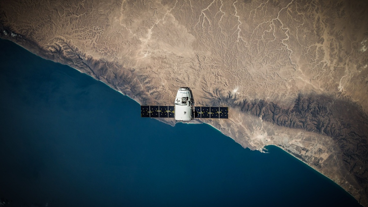
Satellites measure sea-surface salinity indirectly by detecting faint microwave energy emitted by the ocean. The strength of that natural emission changes slightly with salt concentration. Radiometers record the signal, then retrieval algorithms correct for water temperature, surface roughness and other interference before converting it into a salinity estimate.
The measurement covers only the ocean’s uppermost layer, roughly the first centimeter. NASA missions combine repeated wide swaths into regional and global maps. The JPL explanation of SMAP salinity sensing shows how these observations extend the earlier Aquarius record.
No satellite tastes seawater or counts salt crystals. Its advantage is coverage: ships and floats measure accurately at points, while an orbiting sensor revisits nearly the entire ice-free ocean. Scientists compare both kinds of data to reveal changes in the global water cycle.
Warm matter emits microwave energy
Every object above absolute zero emits electromagnetic radiation. At the low microwave frequency used for salinity, the ocean’s brightness temperature depends on its physical temperature and emissivity. Dissolved ions alter the electrical properties of seawater, producing a small but measurable change.
A passive microwave radiometer receives this natural emission without sending a pulse. The salinity sensitivity is subtle, so the instrument requires careful calibration and a large antenna. Radio-frequency interference from transmitters can overwhelm the ocean signal and must be detected or excluded.
L-band microwaves near 1.4 gigahertz are especially useful because atmospheric absorption is low and salinity sensitivity is practical. The long wavelength demands a broad footprint, which limits spatial detail compared with visible cameras.
A retrieval removes other influences
Sea-surface temperature changes microwave emission more strongly than salinity in cold water. Algorithms therefore use independent temperature fields. The correction becomes difficult near freezing, which reduces salinity accuracy at high latitudes.
Wind roughens the surface and adds foam, changing the signal seen from different angles. Aquarius carried a scatterometer to estimate roughness. SMAP uses model winds and related information after the radar portion of its mission stopped operating.
The atmosphere contributes its own emission and attenuation. Galactic radiation can reflect from the sea and the Sun creates contamination at certain viewing geometries. Land is much brighter at these frequencies, so coastlines and islands can affect nearby ocean pixels.
A final salinity retrieval combines these corrections with the calibrated radiometer measurement. Quality flags identify ice, heavy rain or radio interference. Researchers average repeated observations to reduce random noise.
Aquarius proved global mapping was possible
The joint NASA and Argentine Aquarius/SAC-D mission launched in 2011. It flew about 657 kilometers above Earth and produced NASA’s first dedicated global sea-surface salinity maps. The mission completed its primary science goals before ending in 2015.
Aquarius used three passive radiometers and an active scatterometer. NASA reports that it could detect salinity changes of about 0.2 practical salinity units across broad open-ocean areas. Its roughly 150-kilometer spatial resolution favored basin patterns over small coastal features.
The Aquarius mission record links salinity with freshwater exchange and circulation. Repeated maps showed salty subtropical regions, rainy equatorial zones and fresh plumes extending from major rivers.
SMAP continued the record
NASA launched the Soil Moisture Active Passive satellite in 2015 primarily to study land moisture. Its L-band radiometer is also sensitive to ocean salinity. Scientists adapted retrieval methods so SMAP could continue mapping after Aquarius ended.
SMAP has a large rotating antenna and covers broad swaths. Its salinity products are useful for changes over weeks and basin scales. Specialized processing improves coastal resolution, though land contamination remains a challenge near shore.
NASA’s field report on satellites and salinity explains that the mission detects subtle L-band variations. Ship campaigns provide direct samples beneath the satellite track and help test whether the retrieval responds correctly to rain or fronts.
In-water sensors keep the maps accurate
Argo floats measure conductivity and temperature below the surface. Research ships collect water samples and precise CTD profiles. Moorings provide long time series in regions where rapid change can be compared with satellite overpasses.
The satellite footprint may contain many distinct water types, while a float samples one point. Validation therefore accounts for distance, time and the difference between the top centimeter and deeper measurements. Heavy rain can create a fresh skin that a satellite sees before mixing reaches a sensor several meters down.
Biases are tracked across the mission. Calibration updates can lead agencies to reprocess the entire archive, giving users a more consistent climate record. A map’s version and quality flags are important parts of the data.
What salinity maps reveal
Evaporation raises surface salinity, while precipitation lowers it. Satellites provide a global view of this exchange and reveal large river plumes after seasonal floods. They can follow freshwater exported from melting ice, although sea ice itself blocks retrievals.
Salinity affects density and helps control ocean stratification. Combining salinity with temperature and sea-surface height improves studies of currents. During tropical cyclones, a fresh cap can suppress mixing and leave warm water near the surface, although the outcome depends on the full subsurface structure.
Satellite products cannot replace ship or float observations. Their broad coverage complements the precision and depth of in-water instruments. Together they make salinity a routinely observed climate variable rather than a property known only along occasional research cruises.
Limits define the best uses
Satellite salinity works best across the open ocean and over broad time averages. Narrow estuaries are smaller than the sensor footprint and nearby land contaminates the microwave signal. Ice-covered water is unavailable because the radiometer sees ice rather than sea.
Accuracy declines in cold water, where salinity produces a smaller change in brightness temperature. Rain can create electromagnetic interference and a real fresh surface layer. Retrieval flags help users decide whether to include a pixel.
The maps suit basin-scale freshwater transport, seasonal river plumes and large climate patterns. Harbor management or drinking-water decisions need local instruments with finer resolution.
Users should inspect product version, averaging period and uncertainty. A smooth map may combine many noisy observations. Scientific conclusions become stronger when the same feature appears in independent satellite and in-water salinity records.
The indirect method is powerful precisely because its limits are known. It converts a nearly invisible microwave difference into a global view, while direct sampling supplies the chemical ground truth.
From orbit to a published data product
Raw telemetry first becomes calibrated brightness temperature. Processing teams apply antenna-pattern corrections and remove known instrument effects. Geolocation assigns each observation to a point on Earth before the ocean retrieval begins.
A level-two product keeps observations along the satellite swath. Level-three products place them on a regular grid and average across a defined period. Researchers must avoid counting neighboring gridded pixels as independent measurements.
Mission teams validate each release and document changes. Reprocessing with a better correction can alter older maps, which is desirable for a consistent record. Users should cite the product version so another analyst can reproduce the result.
Why repeated coverage is valuable
A research vessel can map a transect precisely, yet conditions change behind it. A satellite returns on a regular schedule and reveals whether a broad feature persists. Repetition is central to measuring seasonal salinity change.
Multi-year coverage also separates recurring cycles from unusual events. When combined with rain estimates and currents, a salinity time series can trace where freshwater entered the ocean and how it spread.
Coverage becomes particularly valuable after major floods or unusual rainfall. A sequence of passes follows the plume beyond the range of coastal stations and helps models estimate freshwater transport across the open sea over time globally.
Related reading: how saltwater lakes form and the saltiest ocean in the world.