Ocean currents are measured in several ways. Some instruments follow water or listen for moving particles, while others scan the sea surface or infer motion from satellites. No single tool captures the whole ocean. Researchers combine ship and anchored-sensor records with drifting floats. Coastal radar and spacecraft extend the view from the shoreline to the deep sea.
The choice depends first on depth and speed. Geographic scale and the desired duration narrow it further. A sensor fixed to the seabed records water passing one point, while a drifter travels with the flow. NOAA’s overview of current monitoring traces the progression from objects timed alongside ships to modern acoustic instruments and satellite-linked platforms.
Drifters follow the water
A surface drifter usually consists of a float, a transmitter and a submerged drogue that catches the moving water below the waves. Satellites determine the drifter’s position at regular intervals. The change in position divided by elapsed time provides an estimate of current speed and direction along the path.
Wind can push the exposed float differently from the water, so the drogue helps the instrument follow a chosen depth more faithfully. If the drogue is lost, researchers flag the record because wind-driven slippage may increase. The Global Drifter Program maintains a worldwide array for ocean circulation research. Its observations also support weather prediction and studies of drifting material.
Profiling floats work deeper. An Argo float adjusts its buoyancy, descends, drifts at a programmed depth, then rises while measuring properties such as temperature and salinity. Its displacement during the deep drift reveals an average current. The Argo program uses thousands of these robots to sample regions that ships visit only occasionally.
Researchers can also release dye or biodegradable tracers in controlled studies and follow how a patch spreads. A tracer shows both the average movement and mixing that separates neighboring water parcels. Such experiments are limited in area and require careful environmental planning, but they reveal fine-scale processes that a sparse network of drifters may miss.
Current meters record flow at one place
Mechanical current meters use a rotor or propeller whose turning rate changes with water speed. A vane can orient the instrument and show direction. These devices established many early records, but moving parts can foul or wear, especially during long deployments.
Modern moorings often carry electronic sensors at several depths. Electromagnetic meters estimate velocity from the voltage created when conductive seawater moves through a magnetic field. Mooring motion and tilt must be measured because the instrument itself may sway in strong flow.
A fixed meter produces a time series that can reveal tides and storms. Longer records show seasonal shifts, while rapid sampling captures brief pulses. Several instruments arranged across a channel can help estimate transport, meaning the total volume of water passing through a cross-section. Gaps remain between the sensors, so researchers use models and repeated ship surveys to describe the full pattern.
Shipboard measurements add spatial detail. A vessel can cross a current repeatedly or occupy stations along a line. Navigation data must be precise because the ship’s movement is much faster than many currents being measured.
Acoustic profilers measure many depths at once
An acoustic Doppler current profiler, or ADCP, sends sound pulses into the water. Tiny particles and plankton scatter some sound back. Their motion changes the returned frequency through the Doppler effect, allowing the instrument to calculate velocity along each acoustic beam.
Several beams pointed in different directions let an ADCP reconstruct three-dimensional water motion. Travel time separates the water column into depth bins, so one instrument can create a vertical profile rather than one reading. The U.S. Geological Survey describes the same principle in river discharge measurements, where ADCPs measure water velocity and depth from a moving boat.
An ADCP can face upward from the seabed, hang beneath a buoy, or operate from a ship. Bottom-mounted systems may observe a location for months. Ship-mounted units map broad sections, although analysts must correct for vessel speed and heading. Pitch and roll require separate corrections.
Sound works in darkness and cloudy water, but acoustic measurements have limits. Sparse scattering particles can weaken the return. Fish movement or bubbles may contaminate it. The measurable range and resolution also depend on sound frequency: higher frequencies resolve smaller layers but usually do not travel as far.
Researchers compare acoustic data with other instruments and inspect signal quality. Quality control can remove bins near the surface where waves introduce bubbles or near a boundary where echoes interfere. The surviving profile gives a detailed view of how velocity changes with depth.
Coastal radar maps surface currents
High-frequency radar stations send radio waves over the ocean and receive energy scattered from surface waves. The Doppler shift shows whether the wave field is moving toward or away from a station. Two or more sites observing the same area can combine radial measurements into a two-dimensional surface-current map.
A coordinated set of shore stations can cover large coastal regions repeatedly without placing an instrument at every point. The U.S. IOOS high-frequency radar network supports search and rescue as well as spill response. Scientists also use it for circulation studies and model evaluation. Coverage depends on radio conditions and station geometry. Equipment uptime and the presence of suitable ocean waves affect it too.
Satellites reveal circulation from space
Satellites do not usually watch individual parcels of seawater move. Radar altimeters measure sea-surface height relative to a reference surface. Small slopes in sea level reflect pressure differences and away from the equator those differences help scientists calculate broad geostrophic currents balanced by Earth’s rotation.
Other sensors map sea-surface temperature and ocean color. Separate instruments estimate winds or salinity. Tracers such as temperature fronts can outline eddies or boundary currents. NASA’s explanation of sea-surface topography shows how satellite altimeters reveal broad circulation across ocean basins.
Satellite coverage supplies a consistent global view, but clouds obstruct infrared temperature measurements and altimeters sample along orbital tracks. Near coasts, land and complex tides make some products harder to interpret. In-water instruments supply depth and calibration that remote sensing cannot provide alone.
Gravimetric satellite missions also improve the reference needed to interpret sea-surface height, while repeated altimeter missions create records spanning decades. Oceanographers remove tides and atmospheric pressure effects when the goal is longer-term circulation. For a storm or coastal flood study, those rapidly changing signals may instead be central to the analysis.
Measurements become useful through combination
Ocean models blend physical equations with observations. Data assimilation adjusts a model toward measured conditions while preserving a dynamically consistent estimate between instruments. Forecast systems can then project currents for navigation and emergency response. Scientists also use the projections to plan fieldwork.
Agreement between independent methods builds confidence. A drifter path can be compared with radar at the surface, while an ADCP reveals the flow underneath. Satellite height can place the local record within a basin-scale eddy. Differences may uncover sensor problems or real motion that one method cannot resolve.
Current speed is commonly reported in meters per second, centimeters per second, or knots. Direction may describe where water is going, unlike wind convention, which often names where air comes from. Metadata must identify depth and the averaging interval. Instrument settings and quality flags are equally important when interpreting the velocity.
Sampling frequency determines what a record can resolve. Hourly averages may describe a tidal cycle but conceal turbulent bursts lasting seconds. A short deployment can capture a storm without revealing seasonal circulation. Researchers match the instrument and deployment duration to the physical question, then select an averaging interval. They archive raw or minimally processed observations so later users can assess those choices.
Repeated calibration and overlapping platforms keep a current map tied to measurements rather than to the assumptions of any one instrument.
Related reading: the Atlantic overturning circulation and how the Gulf Stream was first mapped.