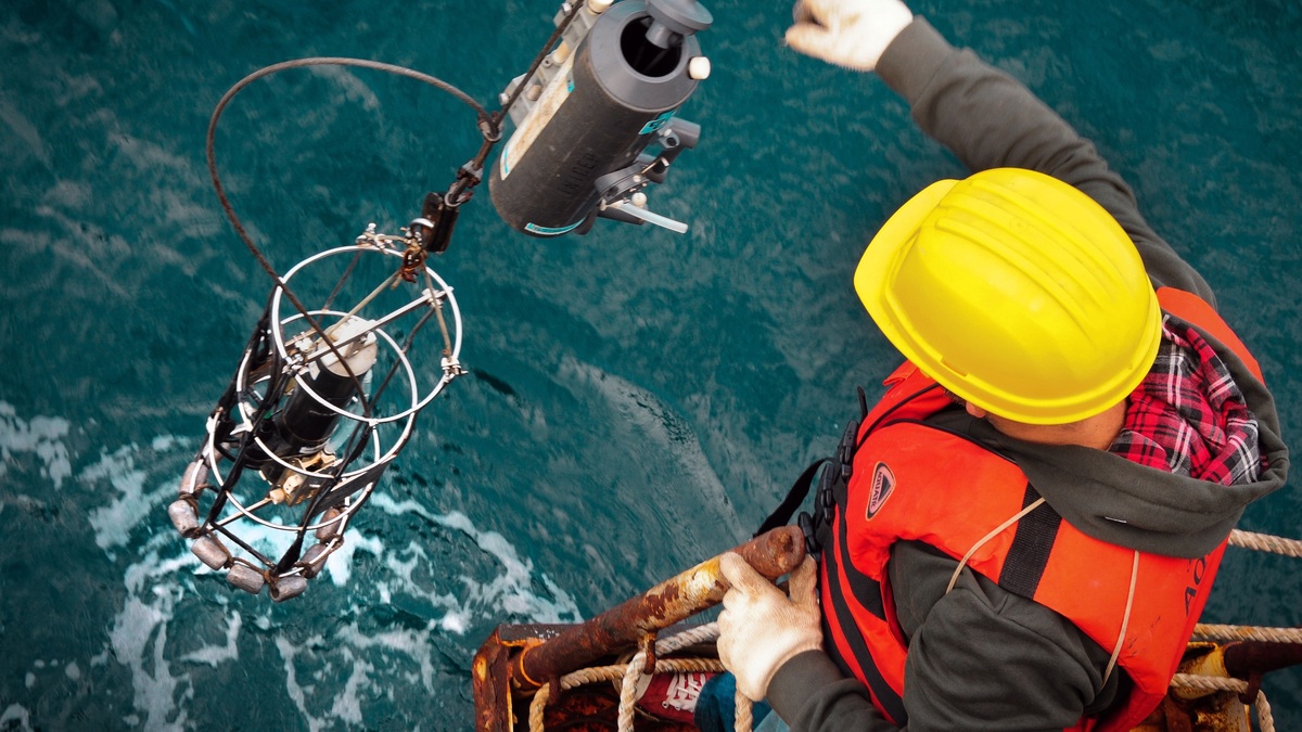
Scientists measure ocean currents with mechanical and electronic current meters, drifting buoys, ship surveys, moorings, satellites and autonomous vehicles. One of the most versatile tools is the acoustic Doppler current profiler, or ADCP, which uses sound to measure water velocity at many depths at once.
No single instrument captures every current. A mooring records change through time at one place, while a ship maps a larger area during a limited visit. Drifters follow moving water near a chosen depth. Satellites infer broad surface flow from sea-surface height and other properties.
A current survey starts with a sampling plan
Researchers first define the scale of motion they need to observe. A tidal inlet may require measurements every few minutes across a channel. A basin-scale climate study may depend on repeated sections and long records. The planned duration must separate tides, weather-driven events and seasonal circulation.
NOAA describes a current survey as a program of observations that determines current speed and direction. Survey design considers water depth, navigation needs and the expected variability of the flow.
Position and timing are recorded with the velocity. Depth, wind, waves, temperature and salinity often accompany the current data because each helps explain why the flow changed. Quality control identifies instrument motion, acoustic interference and periods when the sensor could not sample reliably.
ADCPs read the Doppler shift in sound
An ADCP transmits sound pulses along several angled beams. Small particles and plankton scatter part of the sound back. If the scatterers move relative to the instrument, the echo frequency shifts through the Doppler effect. The instrument converts those shifts into velocity along each beam.
Combining measurements from multiple beams produces three-dimensional water velocity. The ADCP divides the water column into depth cells, often called bins and reports a velocity for each one. The result is a profile rather than a single point measurement.
The U.S. Geological Survey explains how a boat-mounted ADCP measures discharge while crossing a river. Oceanographers use the same physical principle from ships, bottom frames, surface buoys and autonomous platforms.
The particles are assumed to move with the surrounding water. Strong swimming by organisms or sediment settling can add bias under some conditions. Good surveys compare beam quality and echo strength, then flag cells where the assumption or signal is unreliable.
Moving boats map a cross-section
A downward-looking ADCP mounted on a vessel can collect profiles continuously as the boat crosses a channel. Navigation data locate each profile. Software combines water velocity with the boat’s motion to build a cross-section of flow.
Bottom tracking uses echoes from the bed to estimate the vessel’s movement. If the bed sediment itself is moving, bottom track can be biased, so an independent satellite-navigation solution may be needed. Pitch, roll and heading sensors correct the beam geometry as the vessel moves.
USGS technical guidance on moving-boat ADCP measurements identifies unsampled zones near the surface, instrument and bed. Side-lobe interference prevents trustworthy velocity estimates close to the bottom and the transducer’s blanking distance creates another gap.
Moorings reveal change through time
An upward-looking ADCP fixed near the seabed can record currents through most of the water column for months. Repeated profiles reveal tidal cycles, storm responses and seasonal shifts. A downward-looking instrument can hang below a buoy or platform when bottom deployment is impractical.
Long deployments trade spatial coverage for temporal detail. Biofouling, battery life and memory limit the record, while fishing gear or strong currents can damage a mooring. Recovery allows scientists to download the complete dataset and apply post-processing corrections.
Fixed measurements are particularly valuable for distinguishing predictable tidal currents from wind-driven flow. A month or more of observations can resolve major tidal constituents. Multi-year stations then reveal unusual events against a stable baseline.
Argo’s explanation of current ocean conditions reflects why operational systems combine observations with models. A mooring supplies a local truth point, while a numerical forecast fills gaps between stations.
Drifters and floats move with the ocean
Surface drifters carry a satellite transmitter and a drogue extending below the waves. The drogue helps the instrument follow water rather than wind acting directly on the float. Its changing position gives a Lagrangian view, meaning the measurement follows the moving fluid.
Profiling floats adjust buoyancy, descend and later rise while measuring temperature and salinity. Their drift at parking depth provides information about subsurface circulation. The global Argo program maintains thousands of such floats, supplying broad coverage that ships alone could not sustain.
Gliders use small buoyancy changes and wings to move forward through the water. Their repeated dives create sections across fronts or along coasts. Onboard navigation and estimated motion through water can supplement direct current measurements.
Satellites infer broad surface flow
Radar altimeters measure sea-surface height from orbit. After corrections for waves, atmosphere and tides, horizontal slopes in the sea surface reveal pressure gradients. Away from the equator and coasts, those gradients can be used to estimate geostrophic surface currents.
Satellite-tracked sea-surface temperature and ocean color expose fronts, eddies and filaments that move with currents. These images trace patterns rather than directly measuring all velocity. Combining them with altimetry, drifters and models produces a more complete map.
Argo’s overview of ocean currents and climate shows why coverage across both space and time is essential. Heat transport cannot be calculated from one current meter; it requires velocity plus temperature over a large section.
Every measurement contains limits
ADCPs need sufficient acoustic scatterers and cannot sample immediately beside the transducer or bed. Drifters may lose their drogues. Satellites mainly observe the surface and may struggle near coastlines. Moorings can miss an eddy passing a short distance away.
Scientists manage these limits through overlapping methods. A ship survey provides detailed calibration, a mooring supplies continuity and remote sensing supplies geographic context. Models integrate the observations while preserving physical laws, then identify where new measurements would reduce uncertainty.
Ocean-current measurement is therefore a network rather than a single device. The ADCP is central because it rapidly profiles velocity through depth, but its best results come when position, hydrography and independent observations are considered alongside the echoes.
How velocity becomes transport
Current speed at one point does not reveal how much water a current carries. Volume transport requires velocity integrated across the current’s width and depth. Oceanographers repeat sections so they can measure the changing shape of a jet rather than extrapolate from its fastest core.
Temperature and salinity profiles convert transport into heat or freshwater transport. The calculation needs a reference and careful accounting of flow in both directions. Small velocity biases across a large section can produce a large error in the final total.
For rivers, discharge is the cross-sectional integral of downstream velocity. A moving-boat ADCP estimates it during repeated transects. In the ocean, open boundaries and moving water masses make the equivalent calculation more complex, but the same principle of summing velocity over area applies.
Uncertainty is reported alongside the estimate. Instrument precision, unsampled edges, navigation error and natural variability all contribute. Repeated measurements show whether an apparent change exceeds those limits.
Calibration protects the final result
Calibration includes checking transducer alignment and the compass. A small heading error rotates every measured vector, which can bias transport across a section. Test runs over a known course and comparison with independent navigation expose problems before a long deployment.
Data processing preserves both the cleaned result and the original observations. Researchers document excluded bins and correction choices so another analyst can reproduce the calculation. A smooth color plot may look convincing even when the acoustic signal was weak, making transparent quality flags essential.